Introduction
In this post we will consider a probability problem that is so simple we can find its solution after a moment’s thought. We will then over-engineer that solution in terms of mathematical rigour, and finally show how that mathematical model can be translated in a one-to-one fashion into R code. We will then use that code to simulate the problem and see if it matches our earlier solutions.
Problem
(I found this problem on Brilliant, which is a fun app and website for doing math problems.)
Consider a factory producing 1,000 widgets per day. Any given widget has a 1% probability of being defective. After the widget is produced it goes through a quality assessment. A defective widget has a 1% probability of erroneously passing this assessment, while a non-defective widget has a 2% probability of erroneously not passing this assessment.
On average, how many mistakes does the quality assessment do per day? Assume all widgets are produced and assessed independently of each other.
Intuitive solution
The factory produced 1,000 widgets per day. On average 10 of these are defective (1% of 1,000). Of these defective ones, 0.1 slip through the QA (1% of 10). Meanwhile, 990 non-defective ones are produced, and 19.8 (2% of 990) erroneously get caught in the QA. So on average 19.8 + 0.1 = 19.9 mistakes are made per day.
Rigorous solution
We can model this problem using indicator variables and linearity of expectations. To tie the problem back to the language often used in probability theory, let’s not think of factories and widgets, but rather of scientists and experiments. So the factory is like a scientist and producing a widget is like conducting an experiment. The outcome of that experiment can be one of four possibilities:
- A defective widget getting caught in QA
- A defective widget not getting caught in QA
- A non-defective widget getting caught in QA
- A non-defective widget not getting caught in QA
This is our sample space. If we denote defectiveness by \(D\) and getting caught in QA by \(C\), then we can write the sample space as the cartesian product of the sets \(\{D, \neg D\}\) and \(\{C, \neg C\}\):
\[ \begin{align} S & = \{ D, \neg D \} \times \{ C, \neg C \} \\ & = \{ (D, C), (D, \neg C), (\neg D, C), (\neg D, \neg C) \} \end{align} \]
Once we have a sample space, we can define random variables on that space to let us work with numbers instead of sets. In particular, let’s define a random variable \(I\) in the following way:
\[ I \colon S \to \{0,1\} \\[10pt] \] \[ \begin{align} I(D, \neg C) & = I(\neg D, C) & = 1 \\ I(D, C) & = I(\neg D, \neg C) & = 0 \end{align} \]
That is, \(I\) takes as input an outcome of the experiment (e.g. a non-defective widget that gets caught in QA \((\neg D, C)\)) and returns either a 1 or a 0. We call this an indicator random variable for the obvious reason: it returns a 1 if a mistake was made, and 0 otherwise.
We can now define a second random variable \(X\) to represent the number of mistakes made in a day. To be really pedantic about its definition, let’s define it in the following way:
\[ X \colon S^{1000} \to \mathbb{Z} \\[10pt] X(x) = I(x_1) + I(x_2) + \dots + I(x_{1000}) \\[10pt] \text{where } x_n \text{ is the nth ordered pair of the 1000-tuple } x. \]
That is, \(X\) takes as input a 1000-tuple of ordered pairs and returns an integer. We get that integer by applying our indicator variable \(I\) to each pair and summing up their values. Intuitively, we produce 1000 widgets, check each one if a mistake was made in the QA process, and count the number of mistakes.
To be less pedantic, we can also just say that \(X = I_1 + I_2 + \dots + I_{1000}\) and not explicitly acknowledge the fact that \(X\) is a variable with a domain and codomain.
Now, the question asks for the average number of mistakes in a day. In our model, this corresponds to the expected value of the random variable \(X\). Hence,
\[ \begin{align} E(X) & = E(I_1 + I_2 + \dots + I_{1000}) && \text{variable substitution} \\ & = E(I_1) + E(I_2) + \dots + E(I_{1000}) && \text{linearity of expectations} \\ & = E(I) + E(I) + \dots + E(I) && \text{all } I_i \text{ are i.i.d} \\ & = 1000 E(I) && \text{definition of products} \\ & = 1000 \sum_{x \in \{0,1\}} I(x) P(I = x) && \text{definition of expected value} \end{align} \]
So if we could just evaluate that last expression – \(\sum_{x \in \{0,1\}} I(x) P(I = x)\) – we’re done. Evaluating the \(P(I = x)\) part gives us:
\[ \begin{align} P(I = 1) & = P( \{ s \in S \mid I(s) = 1 \}) && \text{definition of random variable equality} \\ & = P(\{ (D, \neg S), (\neg D, S) \}) && \text{evaluating the set comprehension} \\ & = P(\{ (D, \neg S) \} \cup \{ (\neg D, S) \}) && \text{disjoint sets} \\ & = P(\{ (D, \neg S) \} ) + P( \{ (\neg D, S) \}) && \sigma \text{ additivity} \\ & = P(D) P( \neg S) + P( \neg D ) P(S) && \text{multiplication rule for independent events} \\ & = .01 \times .01 + .99 \times .02 && \text{by assumption} \\ & = .0001 + .0198 && \text{arithmetic} \\ & = .0199 && \text{arithmetic} \end{align} \]
The corresponding calculation for the case \(I = 0\) yields:
\[ \begin{align} P(I = 0) & = .01 \times .99 + .99 \times .98 \\ & = .0099 + .9702 \\ & = .9801 \end{align} \]
Hence:
\[ \begin{align} \sum_{x \in \{0,1\}} I(x)P(I = x) & = 1 \times P(I = 1) + 0 \times P(X = 0) \\ & = 1 \times .0199 + 0 \times .9801 \\ & = .0199 \end{align} \]
Continuing on from where we left off earlier:
\[ \begin{align} E(X) & = 1000 \sum_{x \in S} I(x) P(I = x) \\ & = 1000 \times .0199 \\ & = 19.9 \end{align} \]
And so we’ve arrived at the same answer as we got through our intuitive reasoning earlier.
R simulation
As a final check on our answer, let’s simulate the problem in R, paying specific attention to making the code mirror the mathematics as closely as possible.
We define our indicator variable \(I\):
I <- function(defective, selected) {
  defective & !selected | !defective & selected
}
Again, it takes as input a tuple representing a widget and returns either 0 or 1 (technically it returns a boolean (TRUE/FALSE), but we will coerce this to integers later on).
Next, we set up our sample space \(S\):
is_defective <- function(n, p_def = 0.01) {
  sample(c(TRUE, FALSE), size = n, replace = TRUE,
         prob = c(p_def, 1 - p_def))
}

is_selected <- function(defective, ps = c(0.99, 0.02)) {
  p_sel <- if(defective) ps[1] else ps[2]
  sample(c(TRUE, FALSE), size = 1,
         prob = c(p_sel, 1 - p_sel))
}

is_selected <- Vectorize(is_selected, "defective")

set.seed(1)
is_selected(is_defective(8))
## [1] FALSE FALSE FALSE FALSE FALSE FALSE FALSE FALSEis_defective allows us to produce n widgets, each with a p_def probability of being defective. We can then pass these to is_selected to simulate QA mistakes being made.
Lastly, let’s also define our random variable \(X\):
X <- function(n, p_def = 0.01, ps = c(0.99, 0.02)) {
  d <- is_defective(n, p_def)
  s <- is_selected(d, ps)
  Is <- I(d, s)
  sum(Is)
}

X(1000)
## [1] 15We can now let our factory run for a 1,000 days, producing 1,000 widgets each day.
library(ggplot2)
x <- replicate(1000, X(1000))
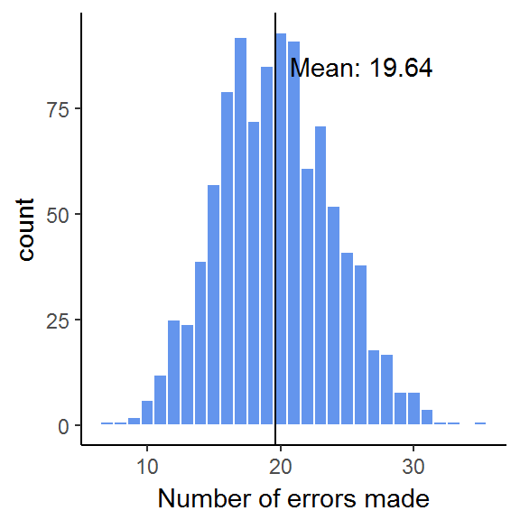
summary(x)## Min. 1st Qu. Median Mean 3rd Qu. Max.
## 7.00 17.00 20.00 19.64 23.00 35.00Indeed, we get a simulated mean very close to our previous results of \(E(X) = 19.9\).
Finally, let’s plot all simulations:
ggplot() +
  geom_histogram(aes(x), binwidth = 1,
                 fill = "cornflowerblue",
                 color = "white") +
  geom_vline(xintercept = mean(x)) +
  annotate("text", x = mean(x), y = 85, hjust = -0.1,
           label = sprintf("Mean: %0.2f", mean(x))) +
  theme_classic() +
  labs(x = "Number of errors made")