Probability kata

Introduction

While having dinner with a colleague last night, my colleague told me that he’d played a dice game with a risk-loving opponent (who also apparently made a lot of money on the Bitcoin bubble). My colleague said that they had each rolled a six-sided die ten times, and that his friend had (correctly!) bet that he would roll higher on all ten rolls. This seemed implausible to me, but exactly how implausible?

In the following we solve the problem exactly, and then confirm our calculations through simulation.

Problem

Two players each roll a six-sided, fair die ten times in a row. What is the probability that Player 1 rolls higher than Player 2 all ten times?

Analytical solution

Let \(\Omega = \{ (x,y) \mid x,y \in \{1, \dots, 6\}\}\) be the sample space, so that \(|\Omega| = 36\). Let \(X_1, X_2 \sim \mathcal{U}(1,6)\) be two random variables representing the rolls of Player 1 and 2 respectively. Let \(I\) be an indicator random variable representing the event that Player 1 wins a roll, i.e. \(P(I) = P(X_1 > X_2)\).

The probability of winning a given roll is straightforward: if Player 1 e.g. rolls a 6, then he wins if and only if \(X_2 \in \{1,2,3,4,5\}\). By the naive definition of probability, then,

\[ P(I | X_1 = 6) = \frac{|\{1,2,3,4,5\}|}{|\Omega|} = \frac{5}{36} \approx 0.14. \]

Since the possible events are disjoint, the Law of Total Probability gives us

where we used the fact that \(\sum_{i = 1}^n i = \frac{n(n + 1)}{2}\) in the fourth equality.

So Player 1 has a 42% chance of winning a given roll.

Now, since all rolls are independent and identically distributed, we can interpret each roll as a Bernoulli trial with \(p = \frac{5}{12}\). Consequently, if we let \(W\) be a random variable representing the total number of rolls won, see that \(W\) is just the sum of \(n = 10\) i.i.d. \(Bern(p)\) trials, i.e. \(W \sim Binom(10, \frac{5}{12})\). By the definition of the Binomial distribution,

\[ P(W = k) = {n \choose k} p^k(1 - p)^{n-k}, \]

we thus have

So the probability of Player 1 winning all ten rolls is about 0.015%.

Verifying analytical solution through simulation

To make sure we made no mistakes in reasoning or arithmetic in the previous section, we will verify our calculations with a simple Monte Carlo simulation.

We define a function roll_dice which samples with replacement twice from a uniform distribution, \(\mathcal{U}(1,6)\). It then checks if the first sample is greater than the second and replicates this process n times.

library(tidyverse)
library(scales)

roll_dice <- function(n = 10) {
  replicate(n, {
  roll <- sample(x = 1:6, size = 2, replace = TRUE)
  roll[1] > roll[2]
})
}

Next, we specify that we’ll run the experiment a million times (n_simulations), and calculate the share of experiments where Player 1 indeed wins all ten rolls.

n_simulations <- 1e6

wins <- replicate(n_simulations, sum(roll_dice()))
table(wins)

## wins
##      0      1      2      3      4      5      6      7      8      9 
##   4432  32973 104644 199544 249365 213785 127425  51612  13911   2156 
##     10 
##    153

cat("\n", "Share of simulations where Player 1 won all ten games:", 
    sum(wins == 10) / n_simulations)

## 
##  Share of simulations where Player 1 won all ten games: 0.000153

Evidently, the simulation results match our earlier calculations to at least five decimal points, so we’re convinced no mistakes were made.

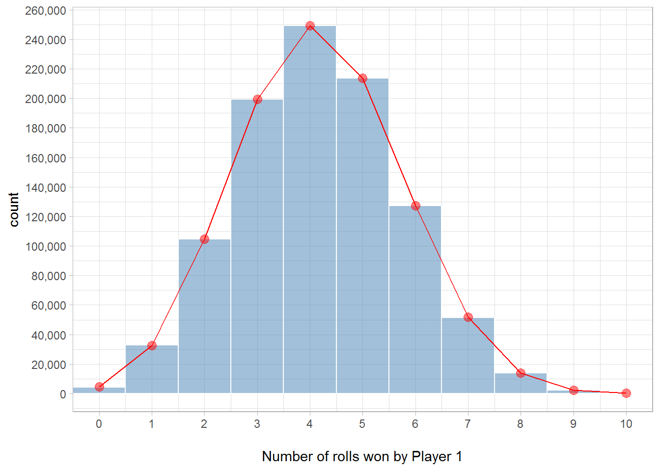
Finally, to confirm that we get the correct results not just for \(k = 10\) but for all \(k \in \{0, \dots, 10 \}\), we can plot the distribution of the number of simulated rolls won by Player 1 and compare this to the probability mass function of the \(Binom(10, \frac{5}{12})\) distribution.

df_binom <- data_frame(wins = 0:10, 
                       y = dbinom(wins, 10, 15/36) * n_simulations)

ggplot(data_frame(wins), aes(x = wins)) +
  geom_histogram(binwidth = 1, color = "white", 
                 fill = "steelblue", alpha = 0.5) +
  geom_line(aes(y = y), df_binom, color = "red") +
  geom_point(aes(y = y), df_binom, size = 3, color = "red", alpha = 0.5) +
  scale_x_continuous(breaks = pretty_breaks(10), expand = c(0, 0)) +
  scale_y_continuous(breaks = pretty_breaks(10), labels = comma) +
  theme_light() +
  labs(x = "\nNumber of rolls won by Player 1")